The Marker Method: Building a Custom Grid for Your Scanned Notes

In my previous post, From Ruled to Unruled: A Digital Eraser for Your Scanned Notes , we built a "digital eraser" and successfully removed ruled lines from images of scanned sheets. We now have a beautifully clean slate to work with, which is a huge win.

But... now what? We have a clean image, but to a computer, it's still just a flat picture of words. A human can easily see the title, the main paragraph, and maybe a list on the side. How do we teach our program to see that same structure?

This is where we get clever. Instead of relying on complex layout analysis algorithms, which can be a real headache, we'll use a simple system of annotations. Our secret weapon is a custom, hand-drawn symbol: two short, parallel lines slanted at about 45 degrees, like a tilted equals sign. By looking for this specific, unnatural shape, we can reliably find our markers without confusing them with actual handwriting.

The strategy:

Scan the clean image to find all pairs of parallel, slanted lines that form our custom markers.
Use their coordinates to create a custom grid overlay on the page.
Intelligently merge the resulting grid cells into larger, meaningful boxes that perfectly contain our notes.

By the end, we won't just have an image; we'll have a structured map of our content, ready for the final step of extraction and OCR. Let's start decoding those markers!

The Methodology: How It All Works

This process might seem complex, but it's really a series of logical filters. We start by finding every possible line on the page and then progressively narrow it down until we're left with only our specific markers. Let's walk through it.

Step 1: Finding All Potential Lines

First, we need to find every straight line in the image. The perfect tool for this is the Hough Line Transform. Think of it as a voting process: for every edge pixel in the image, the algorithm draws all possible lines that could pass through it. The lines that get the most "votes" (i.e., the ones that align with the most edge pixels) are the ones it detects.

We use the probabilistic version, HoughLinesP, which is faster and gives us the start and end points of each line.

def detect_slanted_markers_hough(image, config):
    gray = cv2.cvtColor(image, cv2.COLOR_BGR2GRAY)
    binary = cv2.adaptiveThreshold(
        ~gray, 255, cv2.ADAPTIVE_THRESH_GAUSSIAN_C, cv2.THRESH_BINARY, 15, -2
    )
    lines = cv2.HoughLinesP(
        binary,
        1,
        np.pi / 180,
        config["hough_threshold"],
        minLineLength=config["hough_min_line_length"],
        maxLineGap=config["hough_max_line_gap"],
    )

After getting a big list of lines, we immediately filter them. We're only interested in lines that could be part of our marker. This means they must:

Have the right angle: We're looking for lines around 45 degrees.
Have the right length: They can't be too long or too short.

This first pass dramatically reduces the number of candidates we have to worry about.

Step 2: Pairing Lines to Form Markers

Now for the clever part. A single slanted line isn't a marker; we need two of them that are close and parallel. We loop through our list of candidate lines and try to find a "best friend" for each one.

A good pair of lines must satisfy several geometric conditions:

Similar Length: They should be roughly the same size.
Similar Angle: They must be nearly parallel.
Close Proximity: They can't be too far apart. We measure the perpendicular distance between them to check this.
Correct Alignment: They should be positioned side-by-side, not end-to-end. We check this by making sure their longitudinal distance (the distance along their direction of slant) is small.

The code calculates these distances and finds the best possible partner for each line. If a good match is found, we calculate the midpoint between the two lines' midpoints—this becomes the official coordinate of our detected marker.

# (Inside the loop that pairs lines)
midpoint_dist = math.sqrt(...)
perp_dist = abs(A * x + B * y + C) / math.sqrt(A**2 + B**2)
longitudinal_dist = math.sqrt(midpoint_dist**2 - perp_dist**2)

if perp_dist < min_dist: # and other conditions are met
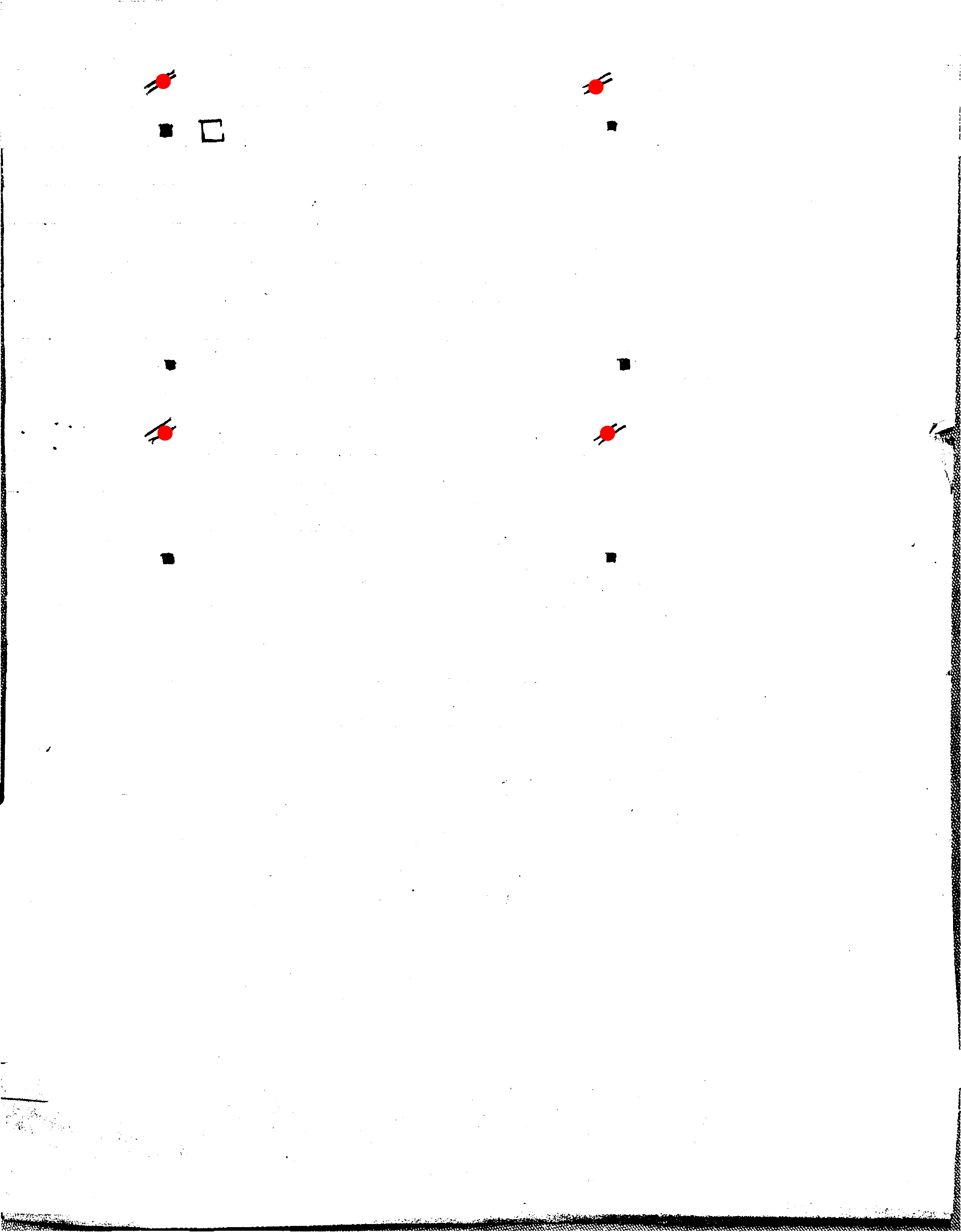
    # We have a potential match!

This is our first pass. The image shows every single marker candidate that our pairing logic found. You'll likely see tight clusters of orange dots where you only drew one marker. This "noise" is expected and shows why the next step is so important.

Step 3: Cleaning Up with Non-Maximum Suppression (NMS)

The Hough Transform can be a bit too enthusiastic. Sometimes it detects multiple, slightly different lines for the same hand-drawn stroke. This means we might end up with a tight cluster of markers where we only intended to draw one.

This is where Non-Maximum Suppression (NMS) comes in. It's a fancy term for a simple idea: "thinning out the crowd."

It takes all the markers within a certain radius.
It treats them as a single group or cluster.
It replaces the entire cluster with a single, averaged point right in the middle.

def non_maximum_suppression(markers, radius):
    # ... logic to find clusters ...
    while markers_copy:
        # ... find all markers within `radius` of the current one ...
        # ... average their positions ...
        avg_x = sum([p[0] for p in cluster]) / len(cluster)
        avg_y = sum([p[1] for p in cluster]) / len(cluster)
        final_markers.append((int(avg_x), int(avg_y)))
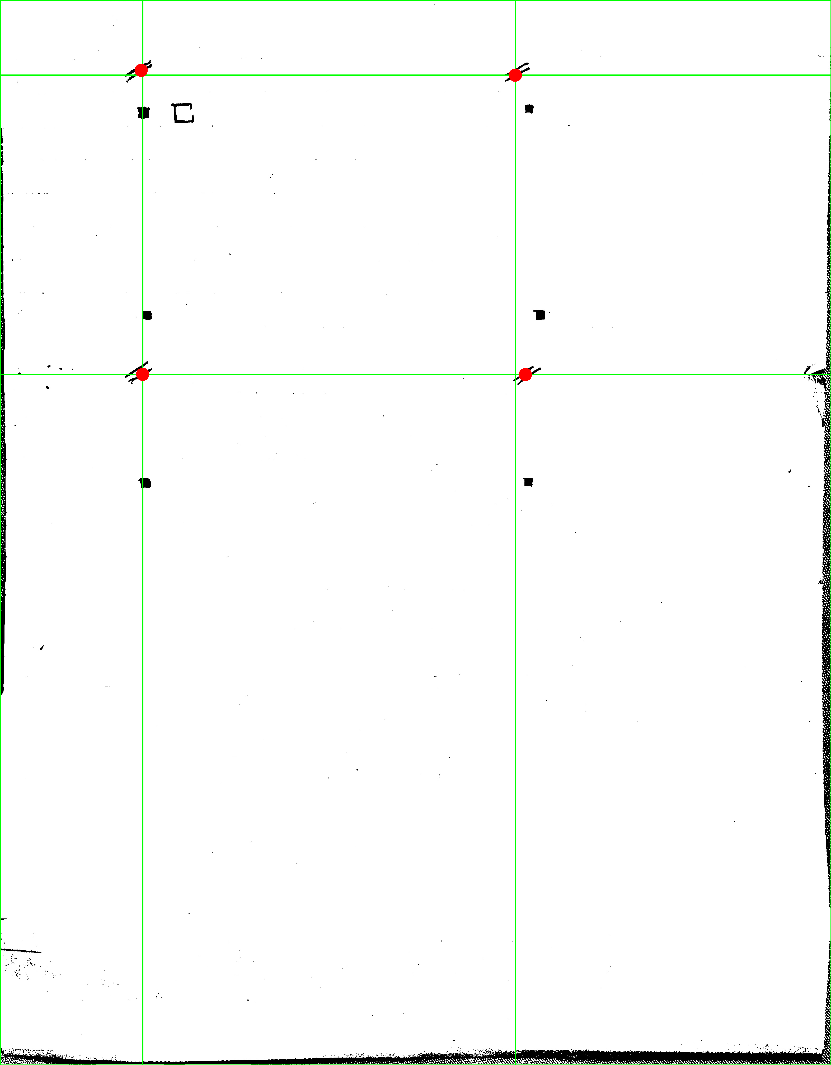
    return final_markers

This ensures that each hand-drawn marker results in exactly one coordinate point. This is the result after Non-Maximum Suppression has done its job. The clusters are gone, and each hand-drawn marker is now represented by a single, clean red dot. This is the clean set of coordinates we'll use to build our grid.

Step 4: From Markers to a Grid

With our clean, final list of marker coordinates, building the grid is straightforward. We collect all the unique X and Y coordinates from our markers. We also add the edges of the image (coordinates 0 and the maximum width/height) to this list.

Then, we draw vertical and horizontal lines through each of these coordinates, effectively creating a grid that spans the entire page and is perfectly aligned with our markers.

h, w, _ = original_image.shape

# --- Generate ALL potential grid lines from markers and image edges ---
x_coords = sorted(list(set([0] + [c[0] for c in final_markers] + [w])))
y_coords = sorted(list(set([0] + [c[1] for c in final_markers] + [h])))

This process creates a set of rectangular cells defined by these grid lines. Here, we take the cleaned marker coordinates and the page edges and draw a grid line through every single one. The result is a highly detailed but overly-segmented grid. You can see how a single large paragraph might be split into several smaller boxes.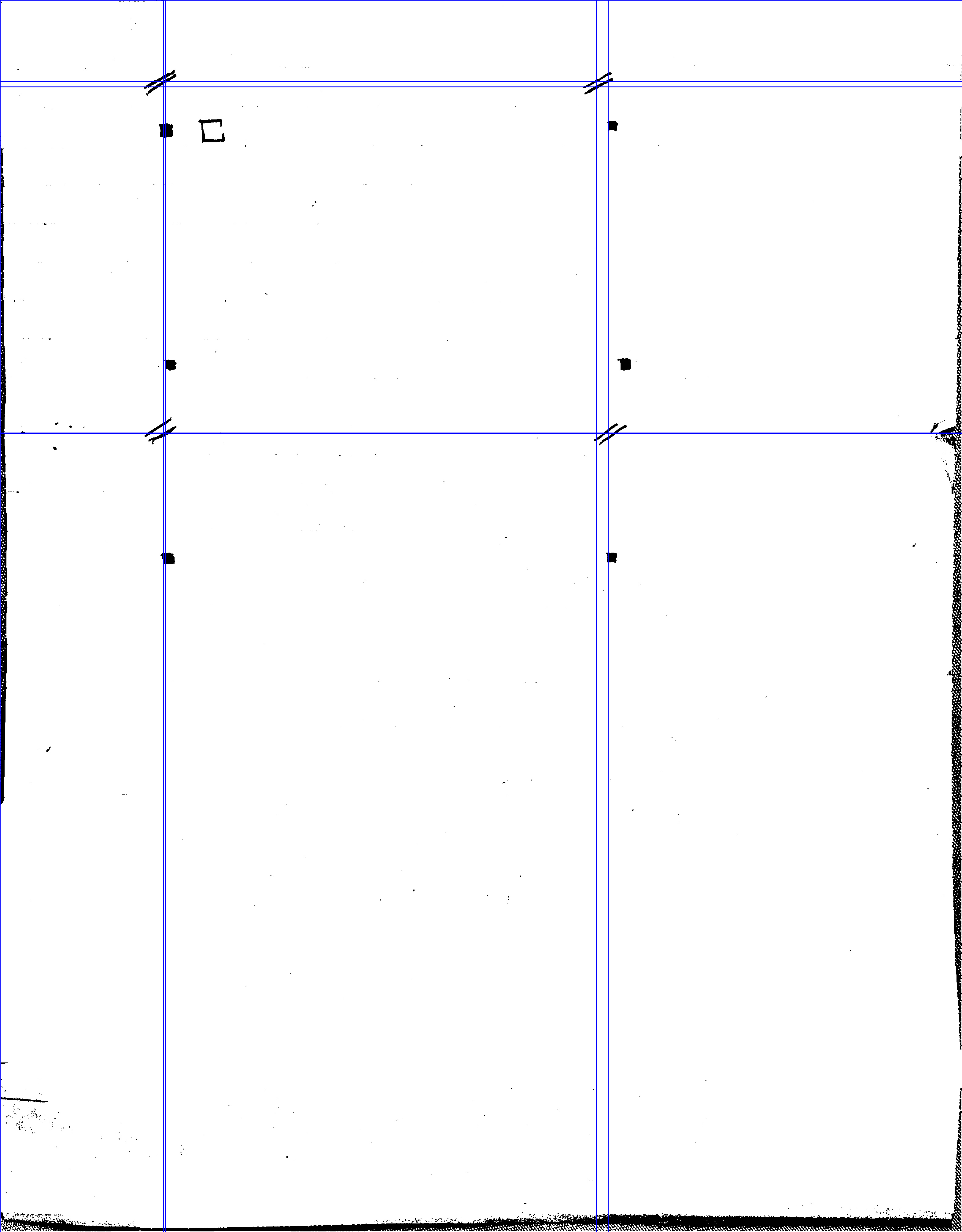

Step 5: Intelligent Box Merging

The grid we just created is too granular. It has lines running through every single marker, resulting in lots of tiny, unnecessary boxes. For instance, a single large paragraph might be diced into four or more small cells.

The final step is to merge these small, impractical boxes into larger, meaningful regions. The logic is simple:

Identify all boxes that are too small (i.e., narrower or shorter than a minimum threshold).
For each small box, find its nearest "large" neighbor.
Merge the small box into that neighbor by creating a new, larger box that encompasses both.

def merge_small_boxes(all_generated_boxes, min_width, min_height):
    # ... logic to identify small and large boxes ...
    for s_item in small_boxes:
        # ... find the nearest large box ...
        # ... create the union of the small and large box ...
        new_x1 = min(s_box[0][0], l_box_current[0][0])
        # ... (and so on for y1, x2, y2)
        # ... update the large box with these new dimensions

This is our final output. The merging algorithm has intelligently combined the small, adjacent cells into larger, more meaningful green rectangles. These boxes now accurately map out the distinct content areas of your notes, just as intended.

After this cleanup, we are left with a set of well-defined rectangular regions that accurately contain the distinct blocks of content on our handwritten page. Success! We now have the structured layout we were looking for.